2.5. Mathematical Plots
- PyPI Package
- Project Home
- Documentation
- Git Repository
- Documentation
- Git Repository
Matplotlib is a comprehensive library for creating static, animated, and interactive visualizations in Python. It consists:
matplotlib.sphinxext.mathmpl: Matplotlib math-text in a Sphinx documentmatplotlib.sphinxext.plot_directive: Matplotlib plot in a Sphinx document
Runtime setup
-
plot_pre_code¶ Code that should be executed before each plot runs will setup over the Sphinx configuration option
plot_pre_code. If not specified or None or empty it will default to a string containing:import numpy as np; from matplotlib import pyplot as plt;.- plot_pre_code
Currently set to:
1
2
3
4
from matplotlib import pyplot as plt
from matplotlib import image as mpimg
from matplotlib import cm
import numpy as np
-
plot_working_directory¶ By default, if None or empty, the
plot_working_directorywill be changed to the directory of the example, so the code can get at its data files, if any. Also its path will be added tosys.pathso it can import any helper modules sitting beside it. This configuration option can be used to specify a central directory (also added tosys.path) where data files and helper modules for all code are located.- plot_working_directory
Currently set to
_images/mplplots.
-
plot_basedir¶ When a path to a source file is given, the Sphinx configuration option
plot_basedirwill respect. It is the base directory, to which.. plot::file names are relative to. If None or empty, file names are relative to the directory where the file containing the directive is.- plot_basedir
Currently set to
_images/mplplots.
2.5.1. Expressions
See the Writing mathematical expressions for lots more information how to writing mathematical expressions in matplotlib.
With matplotlib in Sphinx you can include inline math
 (as role
:mathmpl:`(\alpha^{ic} > \beta_{ic})`) or display math:

-
.. mathmpl::¶ - The example
1
2
3
.. mathmpl::

   \left(\frac{5 - \frac{1}{x}}{4}\right)
- Which gives

2.5.2. Plots
-
.. plot::¶ See the matplotlib Pyplot tutorial and the Gallery for lots of examples of matplotlib plots.
The source code for the plot may be included in one of three ways:
inline content
- the example
1
2
3
4
5
6
7
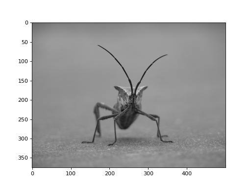
.. plot::
   :align: center
   :scale: 75

   img = mpimg.imread('https://github.com/matplotlib/matplotlib'
                      + '/raw/master/doc/_static/stinkbug.png')
   imgplot = plt.imshow(img)
- which gives
img = mpimg.imread('https://github.com/matplotlib/matplotlib'
                   + '/raw/master/doc/_static/stinkbug.png')
imgplot = plt.imshow(img)
doctest content
- the example
1
2
3
4
5
6
7
8
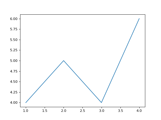
.. plot::
   :format: doctest
   :align: center
   :scale: 100

   >>> import matplotlib.pyplot as plt
   >>> plt.plot([1, 2, 3, 4], [4, 5, 4, 6])  # doctest: +ELLIPSIS
   [<matplotlib.lines.Line2D object at 0x...>]
- which gives
>>> import matplotlib.pyplot as plt
>>> plt.plot([1, 2, 3, 4], [4, 5, 4, 6])
[<matplotlib.lines.Line2D object at 0x...>]

source file content
- the example
1
2
3
4
5
6
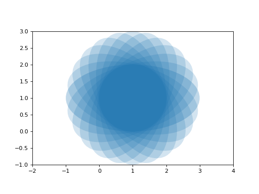
.. plot:: ellipses.py
   :include-source:
   :encoding: utf
   :format: python
   :align: center
   :scale: 100
- which gives
from pylab import *
from matplotlib.patches import Ellipse

delta = 15.0 # degrees

angles = arange(0, 360 + delta, delta)
ells = [Ellipse((1, 1), 4, 2, a) for a in angles]

a = subplot(111, aspect = 'equal')

for e in ells:

    e.set_clip_box(a.bbox)
    e.set_alpha(0.1)

    a.add_artist(e)

xlim(-2, 4)
ylim(-1, 3)

show()

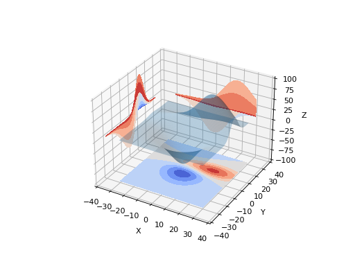
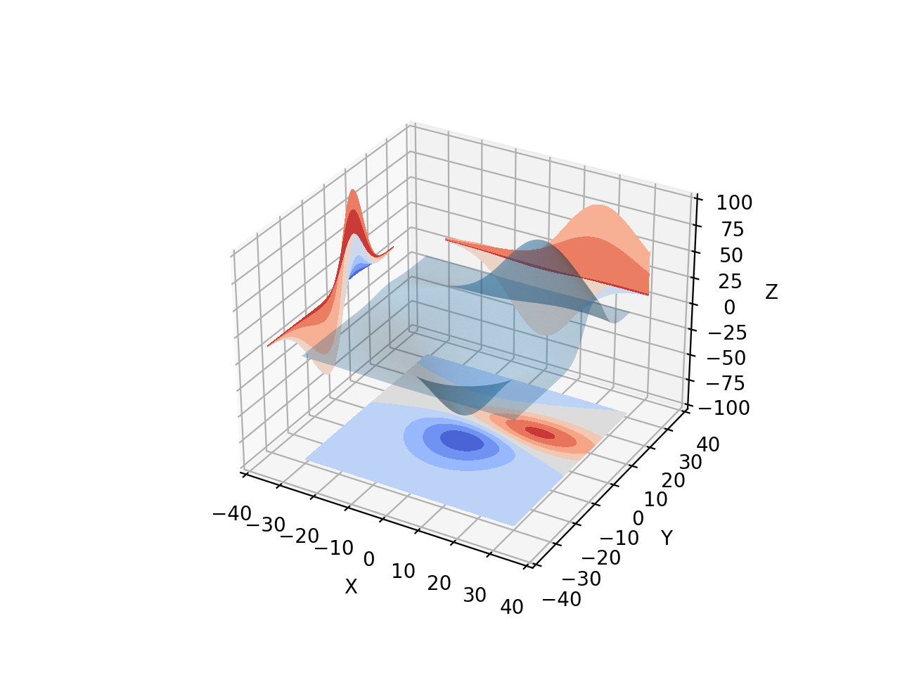
3D-Plots
See mplot3d, mplot3d FAQ, and mplot3d API.
- the example
 1
 2
 3
 4
 5
 6
 7
 8
 9
10
11
12
13
14
15
16
17
18
19
20
.. plot::
   :format: python
   :align: center
   :scale: 100

   from mpl_toolkits.mplot3d import axes3d

   fig = plt.figure()
   ax = fig.gca(projection='3d')
   X, Y, Z = axes3d.get_test_data(0.005)
   ax.plot_surface(X, Y, Z, rstride=8, cstride=8, alpha=0.3)
   cset = ax.contourf(X, Y, Z, zdir='z', offset=-100, cmap=cm.coolwarm)
   cset = ax.contourf(X, Y, Z, zdir='x', offset=-40, cmap=cm.coolwarm)
   cset = ax.contourf(X, Y, Z, zdir='y', offset=40, cmap=cm.coolwarm)

   ax.set_xlabel('X'); ax.set_xlim(-40, 40)
   ax.set_ylabel('Y'); ax.set_ylim(-40, 40)
   ax.set_zlabel('Z'); ax.set_zlim(-100, 100)

   plt.show()
- which gives
from mpl_toolkits.mplot3d import axes3d

fig = plt.figure()
ax = fig.gca(projection='3d')
X, Y, Z = axes3d.get_test_data(0.005)
ax.plot_surface(X, Y, Z, rstride=8, cstride=8, alpha=0.3)
cset = ax.contourf(X, Y, Z, zdir='z', offset=-100, cmap=cm.coolwarm)
cset = ax.contourf(X, Y, Z, zdir='x', offset=-40, cmap=cm.coolwarm)
cset = ax.contourf(X, Y, Z, zdir='y', offset=40, cmap=cm.coolwarm)

ax.set_xlabel('X'); ax.set_xlim(-40, 40)
ax.set_ylabel('Y'); ax.set_ylim(-40, 40)
ax.set_zlabel('Z'); ax.set_zlim(-100, 100)

plt.show()
